LaTeX 作图方法简介

在使用 $\LaTeX$ 做笔记的时候，我们不免要画一些简单的示意图。这里简单介绍两种作图方式，可以很方便的画出简洁而美观的示意图。

TikZ 宏包

在导言区添上 \usepackage{tikz} 后就可以使用 TikZ 宏包了。

画图的代码也很简单，我给出 3 个简单的例子，大家对照代码注释和生成的图看一看就可以了。

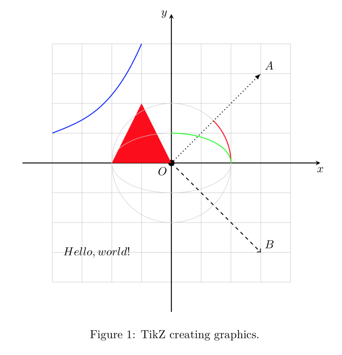
坐标系：

 \begin{figure}[ht]
	
   \centering
   \label{fg:1}
	  
   \begin{tikzpicture}[scale=0.9]
     \draw[step=1,color=gray!40] (-4, -4) grid (4, 4); % 网格 help lines
	    	
     \coordinate (O) at (0, 0);
     \fill (0, 0) circle (3pt); % 画点
     \node[below left] at (O) {$O$};
     \draw[thick, -stealth] (-5, 0) -- (5, 0);
     \draw[thick, -stealth] (0, -5) -- (0, 5);
     \node[below] at (5,0) {$x$};
     \node[left] at (0,5) {$y$};
	
     \fill[red] (0,0)--(-1,2)--(-2,0); % 填充颜色
	
     \draw[color=gray!40] (0,0) circle (2); % (0, 0)代表圆心坐标， 后面 (2) 代表半径
     \draw[thick, color=red] (2,0) arc (0:45:2);	
     % (2, 0)弧的起点坐标，(0:45:2)分别代表始末角度和圆的半径
			
     \draw[color=gray!40] (0,0) ellipse (2 and 1); % 代表半长轴和半短轴
     \draw[thick, color=green] (2,0) arc (0:90:2 and 1);
	
     \draw[thick, blue] (-4,1) .. controls (-3,1.4) and (-2,1.7) .. (-1,4); 
     % 4个点坐标画贝塞尔曲线
	
     \coordinate (A) at (3, 3);
     \draw[thick, dotted, -latex] (0, 0) -- (A);
     \node[above right] at (A) {$A$};
	
     \coordinate (B) at (3, -3);
     \draw[thick, dashed, ->] (0, 0) -- (B);
     \node[above right] at (B) {$B$};
	
     \node at (-2.5, -3) {$Hello, world!$};
   \end{tikzpicture}
	  
   \caption{TikZ creating graphics.}
	  
 \end{figure}

将其编译后生成的图像：

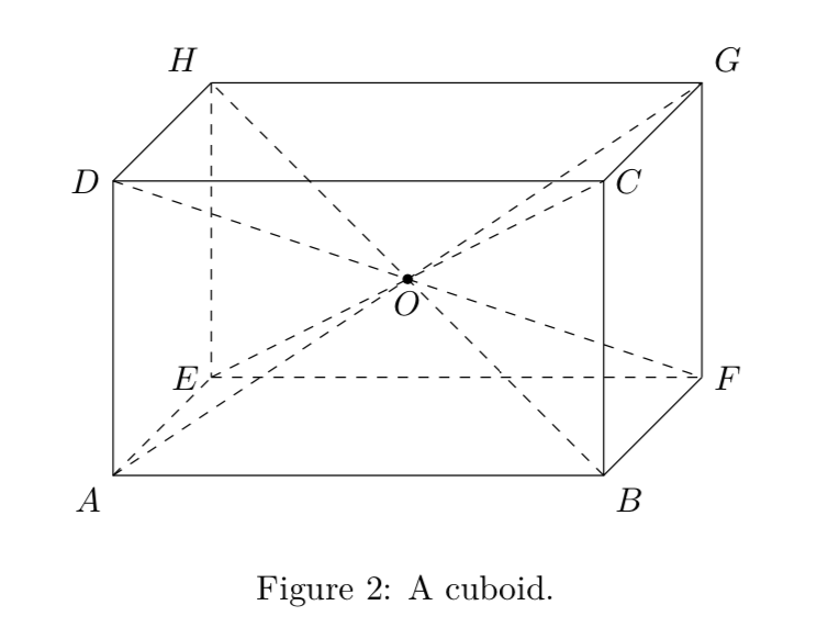
长方体：

 \begin{figure}[ht]
	  
   \centering
   \label{fg:2}
	
   \begin{tikzpicture}
     % 8个顶点
     \coordinate (A) at (0,0) node[below left] at (A) {$A$};
     \coordinate (B) at (5,0) node[below right] at (B) {$B$};
     \coordinate (C) at (5,3) node[right] at (C) {$C$};
     \coordinate (D) at (0,3) node[left] at (D) {$D$};
	
     \coordinate (E) at (1,1) node[left] at (E) {$E$};
     \coordinate (F) at (6,1) node[right] at (F) {$F$};
     \coordinate (G) at (6,4) node[above right] at (G) {$G$};
     \coordinate (H) at (1,4) node[above left] at (H) {$H$};
	
     \fill (3,2) circle (1.5pt) node[below] at (3,2) {$O$};  % 原点
			
     % 12条边
     \draw (A) rectangle (C);
     \draw[dashed] (E)--(F);
     \draw (F)--(G)--(H);
     \draw[dashed] (H)--(E);
     \draw[dashed] (A)--(E);
     \draw (B)--(F);
     \draw (C)--(G);
     \draw (D)--(H);
	
     % 对角线
     \draw[dashed] (A)--(G);
     \draw[dashed] (B)--(H);
     \draw[dashed] (E)--(C);
     \draw[dashed] (D)--(F);
	
   \end{tikzpicture}
	
   \caption{A cuboid.}
	
 \end{figure}

将其编译后生成的图像和教科书上几乎一模一样：

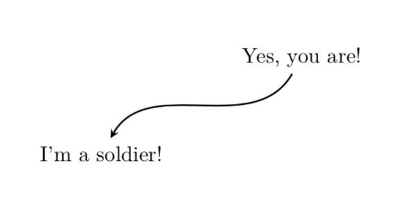
对正文或者公式进行标注：

在导言区添加 TikZ 的位置库和一些设置：

 \usepackage{tikz}
	
 \usetikzlibrary{positioning}	% 可以使用 node 之间的相对位置
 %\tikzset{>=stealth}	% 将 -> 箭头设置为 -stealth

在正文区使用 tikzpicture 环境：

 % 曲线连接
 \begin{tikzpicture}[node distance = 1.5cm]
     \node (A) {I'm a soldier!};
     \node (B) [above right = of A] {Yes, you are!};
     \draw[-stealth, thick] (B) to [in = 60, out = -120] (A);
 \end{tikzpicture}

编译后效果如下：

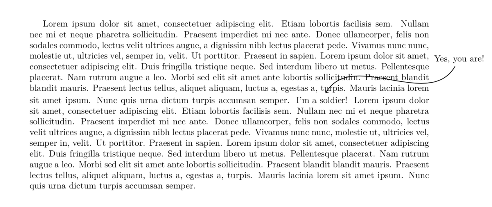
如果想在正文或者公式中添加标注，需要先在导言区定义一个新命令 \tikzmark 用于 mark 被标注的文字或者被标注的公式字母：

 \newcommand{\tikzmark}[3][]			% 在正文或者公式中标记位置
   {\tikz[remember picture, baseline]
     \node [anchor=base,#1](#2) {#3};}

导入 \usepackage{mwe} 宏包后，正文区可以用 \blindtext 随机生成一段文字，中间用 \tikzmark mark 需要标注的文字，在段落结束后紧跟一个 tikzpicture 环境，用 overlay 来使之重叠：

 % 正文标注
 \blindtext	% 随机生成一段文字
 \tikzmark{A}{I'm a soldier!}
 \blindtext
 \begin{tikzpicture}[overlay, remember picture, node distance = 1.5cm]
     \node (B) [above right = of A, xshift = 2.1cm] {Yes, you are!};
     \draw[->,thick] (B) to [in = 60, out = -120] (A);	
 \end{tikzpicture}

效果如下图所示：

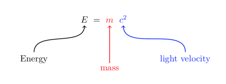
如果想对一个公式进行标注，也是类似的：

 \begin{equation*}
     \tikzmark{node1}{$E$} = \tikzmark[red]{node2}{$m$} \tikzmark[blue]{node3}{$c^2$}
 \end{equation*}
 \begin{tikzpicture}[overlay, remember picture, node distance = 1.5cm]
     \node (node4) [below left=of node1 ]{Energy};
     \draw[->,thick] (node4) to [in=-90,out=90] (node1);
     \node [red] (node5) [below =of node2 ]{mass};
     \draw[red, ->,thick] (node5) to [in=-90,out=90] (node2);
     \node [blue] (node6) [below right =of node3 ]{light velocity};
     \draw[blue, ->,thick] (node6) to [in=-90,out=90] (node3);
 \end{tikzpicture}

效果如下图所示：

Inkscape 作图

Inkscape 是一款跨平台的开源矢量图形编辑软件，和专业的 Adobe Illustrator (AI) 相比，功能虽然少了一些，但是更适合为 $\LaTeX$ 作简图。

在 Inkscape 中绘制好矢量图，将需要的公式用 $\LaTeX$ 表达式写出来，比如 $\int_0^\infty x\mathrm{d}x=0$ ，保存图像时选择 PDF 格式，就会跳出一个选项框，其中的 文字输出选项 选择 忽略 PDF 中的文本并创建 LaTeX 文件，就会生成 xxx.pdf 和 xxx.pdf_tex 两个文件。

在 tex 文件的导言区加入：

 \usepackage{import}
 \usepackage{xifthen}
 \usepackage{pdfpages}
 \usepackage{transparent}
	
 \newcommand{\incfig}[1]{
     \def\svgwidth{0.7\columnwidth}
     \import{./figures/}{#1.pdf_tex}
 }

其中倒数第三行的图像宽度 0.7 可以按需求自行修改。

在 tex 文件的正文区加入：
```
 \begin{figure}[ht]
     \centering
     \incfig{xxx}
     \caption{Inkscape creating graphics.}
     \label{fg:1}
 \end{figure}
```
其中 xxx 是图像文件名 (不带后缀) ，编译后图像文件中的 $\LaTeX$ 表达式就会自动被渲染在图像上，如下图所示：

结语

从此我们就可以用 $\LaTeX$ 画出简洁而美观的示意图了！🎉 🎉 🎉

Go to the Home Page

Sponsor the author if you like the contents!

LaTeX 作图方法简介

简单介绍 2 种 LaTeX 作图方法...

Nov 7, 2019 • Wei Wang

TikZ 宏包

Inkscape 作图

结语